Towards Safe Policy Improvement for Non-Stationary MDPs

Reinforcement learning (RL) methods have shown promise to be applicable to real-world sequential decision-making problems such as medical treatment, budget constrained bidding, and other high-risk high-reward applications. However, to actually deploying RL algorithms for such real-world applications, safety guarantees are critical to mitigate serious risks in terms of both human-life and monetary assets. More concretely, here, by safety we mean that any update to a system should not reduce the performance of an existing system (e.g., a doctor’s initially prescribed treatment). A further complication is that these applications are non-stationary, which violates the foundational assumption of stationarity in most RL algorithms. This raises the main question we aim to address

How can we build sequential decision-making systems that provide safety guarantees for problems with non-stationarities?

In this work, we merge ideas from time-series literature and model-free RL to

• Formalize the safe policy improvement problem for non-stationary MDPs, and provide an algorithm for addressing it.
• Provide a user-controllable knob to set the desired confidence level: the maximum admissible probability that a worse policy will be deployed.
• Develop a method does not require building a model of a non-stationary MDP.

However, our method is designed for environments where changes are smooth and gradual, and might not be ideal for environments where the changes are abrupt.

Problem statement

In a non-stationary setting, the MDP that an agent might face after deployment might be different than the ones it has encountered before. Therefore, in a non-stationary setting we need to ensure safety with respect to the future MDPs that an agent might face. To formalize this, let \(\mathcal D\) be any available historical data and \(\texttt{alg}(\mathcal D)\) be a policy returned by an algorithm after analyzing the data. Let \(\pi^\text{safe}\) be a known safe policy and \((1-\alpha) \in [0,1]\) be the safety level desired by the user. Let \(\rho(\pi, i)\) be the performance of a policy \(\pi\) in episode \(i\) and let \(k\) be the last observed episode number such that episode numbers greater than \(k\) belong to the future. Then we aim to ensure, with high-confidence, that the future performance of the updated policy will provide improvement over the existing \(\pi^\text{safe}\). That is,

\[\begin{align} \Pr \Big(\rho(\texttt{alg}(\mathcal D), {k+\delta}) \geq \rho(\pi^\text{safe}, k + \delta) \Big) \geq 1 - \alpha. \end{align}\]

While it is desirable to ensure the safety guarantee of the form mentioned above, obtaining a new policy from \(\texttt{alg}(\mathcal D)\) that meets this requirement might not be possible unless some more regularity assumptions are imposed on the problem. For example, if the environment can change arbitrarily, then there is not much hope of estimating the future performance to ensure safety.

One way to make the problem more tractable could be to assume Lipschitz smoothness on the dynamics and rewards. However, we show a negative result in the paper and discuss why Lipschitz smoothness might be insufficient for our purpose. Therefore, to make the problem more tractable, we make an alternate assumption that the performance of any policy changes smoothly over time. That is, let \(M_i\) be the MDP in episode \(i\) and let \(\phi\) be a non-linear basis function (like Fourier basis, which is popular for modeling time-series trends) then

Assume: For every policy \(\pi\), there exists a sequence of mean-zero and independent noises \(\{\xi_i\}_{i=1}^{k+\delta}\), and \(\exists w \in \mathbb{R}^{d \times 1}\), such that, \(\forall i \in [1, k+\delta], \,\,\, \rho(\pi, M_i) = \phi(i)w + \xi_i\).

Time-series forecasting and sequential hypothesis testing

To address this problem, we build upon our previous work on non-stationary MDPs, which combines counterfactual reasoning with curve-fitting to estimate the future performance of a policy. That is, for any policy we first estimate its performances on all the past episodes using off-policy evaluation. This univariate sequence of performance estimates are then analyzed to make a performance forecast based on the trend resulting due to the underlying non-stationarity (see here for a short blogpost on that work).

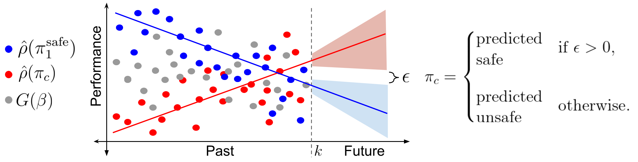
The figure above summarizes the main idea, where \(\pi_c\) is a candidate policy which could potentially be used to provide improvement over \(\pi^\text{safe}\). The gray dots correspond to the returns, \(G(\beta)\), observed for any behavior policy \(\beta\) that was used to collect the data. The red and the blue dots correspond to the counterfactual estimates, \(\hat \rho(\pi_c)\) and \(\hat \rho(\pi^\text{safe})\), for performances of \(\pi_c\) and \(\pi^\text{safe}\), respectively, in different episodes. The shaded regions correspond to the uncertainty in future performance. If we could estimate this uncertainty by analysing the trend of the counterfactual estimates for the past performances, then we could check whether the lower bound on \(\pi_c\)’s future performance is higher than the upper bound on \(\pi^\text{safe}\)’s future performance or not? If it is indeed higher, then we can say with high-confidence that \(\pi_c\) will be safe, otherwise we can say that we do not have enough confidence to provide a safe update and therefore just re-execute \(\pi^\text{safe}\).

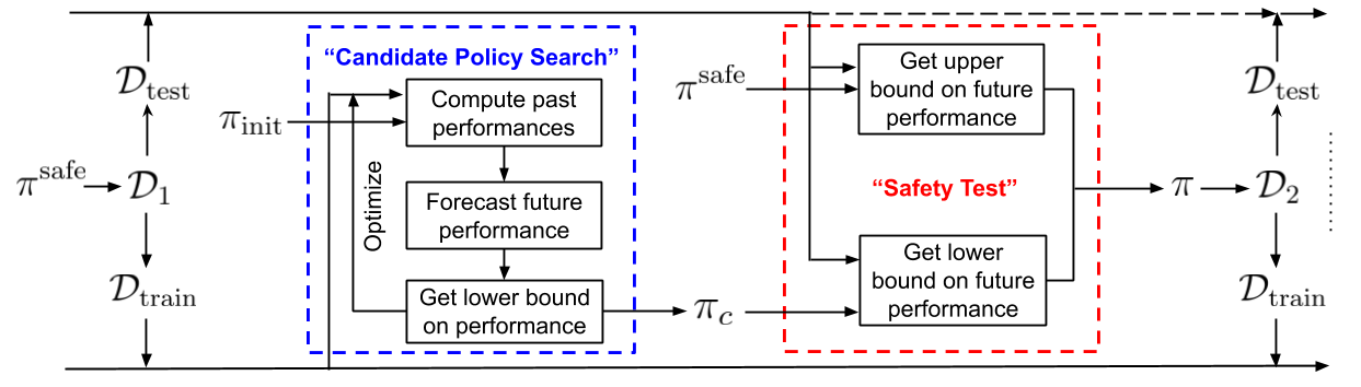
Given a procedure to obtain uncertainty in a policy’s future performance, the above diagram depicts the steps of the proposed algorithm to ensure safety in the presence of non-stationarity. These steps build upon the template for Seldonian algorithms and perform sequential hypothesis (A/B) testing. That is, the proposed algorithm first partitions the initial data \(\mathcal D_1\) into two sets, namely \(\mathcal D_\text{train}\) and \(\mathcal D_\text{test}\). Subsequently, \(\mathcal D_\text{train}\) is used to search for a possible candidate policy \(\pi_c\) that might improve the future performance, and \(\mathcal D_\text{test}\) is used to perform a safety test on the proposed candidate policy \(\pi_c\). The existing safe policy \(\pi^\text{safe}\) is only updated if the proposed policy \(\pi_c\) passes the safety test, and this process continues…

Uncertainty estimation

The above discussion of the main idea relies upon a method to quantify uncertainty in a policy’s future performance. Quantifying this uncertainty requires a careful consideration of the following three factors.

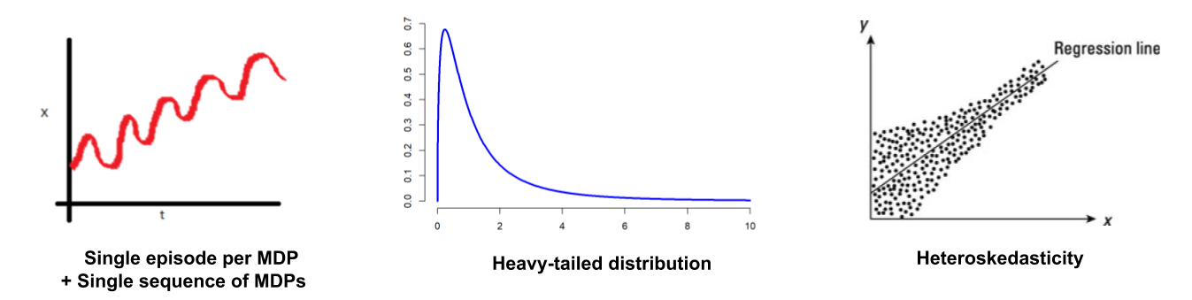
• Single sequence of MDPs: Notice that we only get to observe a single sequence of MDPs. Further, since the MDP can change after every episode due to the underlying non-stationarity, only a single episode per MDP might be available.
• Heavy-tailed distributions: Recall that the off-policy estimation of a policy’s performance requires the use of importance sampling that can lead to extremely heavy-tailed and asymmetric distributions.
• Heteroskedasticity: Since the executed policy can be different for different MDPs in the past, the behavior policy \(\beta\) for importance sampling may be different for different episodes. This results in heteroskedasticity, which is further exacerbated by the changes in the sources of stochasticity as the MDPs change over episodes.

Wild bootstrap

To quantify uncertainty in the future performance while accounting for the above factors, we leverage a technique known as Wild bootstrap from the time-series literature. This allows construction of upto \(2^k\) similar sequence of past performances from a single sequence of the original \(k\) performance estimates, and also tackles heteroskedasticity and non-normal distributions! Having obtained this set of similar sequences of past performances, we first compute an empirical distribution of future performances from it and then consequently obtain the required upper and lower bounds for the future performance. Further, under certain regularity conditions, we show in our paper that the bounds on the future performance obtained using wild-bootstrap are consistent. We outline the steps for this procedure using wild-bootstrap below:

1. Let \(Y^+ := [\rho(\pi, 1), ..., \ \rho(\pi, k)]^\top \in \mathbb{R}^{k \times 1}\) correspond to the true performances of \(\pi\). Create \(\hat Y = \Phi(\Phi^\top \Phi)^{-1}\Phi^\top Y\), a least-squares estimate of \(Y^+\), using the counterfactual performance estimates \(Y := [\hat \rho(\pi, 1), ..., \ \hat\rho(\pi, k)]^\top\) and obtain the regression errors \(\hat \xi := \hat Y - Y\).

2. Create pseudo-noises \(\xi^* := \hat \xi \odot \sigma^*\), where \(\odot\) represents Hadamard product and \(\sigma^* \in \mathbb{R}^{k \times 1}\) is Rademacher random variable (i.e., \(\forall i \in [1,k], \,\, \Pr(\sigma_i^*=+1) = \Pr(\sigma_i^*=-1) = 0.5\)).

3. Create pseudo-performances \(Y^* := \hat Y + \xi^*\), to obtain pseudo-samples for \(\hat Y\) and \(\hat \rho (\pi, {k+\delta})\) as \(\hat Y^* = \Phi(\Phi^\top \Phi)^{-1}\Phi^\top Y^*\) and \(\hat \rho (\pi, {k+\delta})^* = \phi(k+\delta)(\Phi^\top \Phi)^{-1}\Phi^\top Y^*.\)

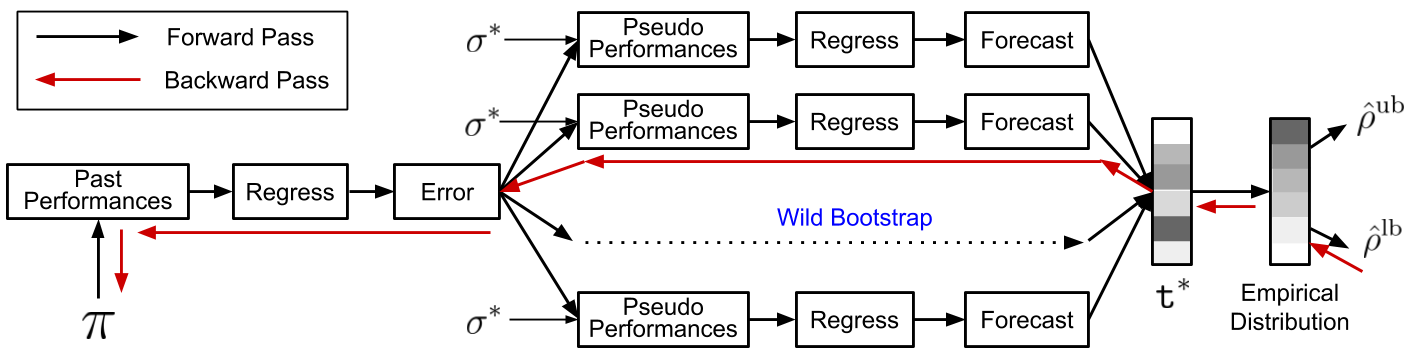
The above image provides a computational graph for quantifying the uncertainty in the forecasted performance. Wild bootstrap leverages Rademacher variables \(\sigma^*\) and the errors from regression to repeat steps 2 and 3 above to create pseudo-performances. Based on these pseudo-performances, an empirical distribution and thus also the lower bound \(\hat \rho^\text{lb}\) for the future performance is obtained. We also show in our paper how the derivative of this lower bound \(\hat \rho^\text{lb}\) with respect to the policy parameters can be computed to search for a candidate policy \(\pi_c\) that maximizes the lower bound. Such a candidate policy will then have the highest chances of passing the safety test and providing a safe policy update.

Empirical performance

We provide an empirical analysis on two simulated domains inspired by safety-critical real-world problems that exhibit non-stationarity. One is for the treatment of Type-1 diabetes and the other is for a recommender system. To understand the impact of different rates of non-stationarity, we conduct the experiment for varying degrees of speed, where speed of 0 represents stationary environment and higher speeds indicate quicker changes in the environment.

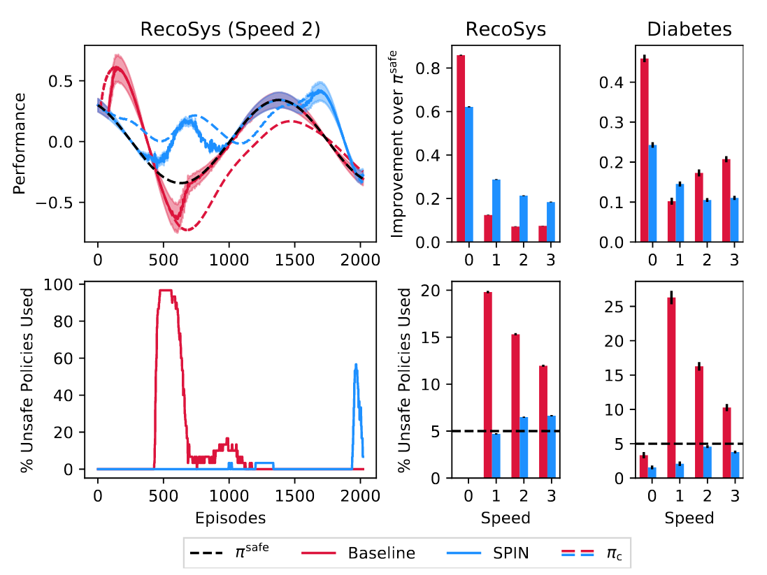
The above figure illustrates the safety violation rates and performances for the proposed method, SPIN, and a baseline safe policy improvement method that does not account for non-stationarity. Top-left plot illustrates a typical learning curve, where it can be noticed that SPIN updates a policy whenever there is room for a significant improvement over the (unknown) performance of \(\pi^\text{safe}\). In the middle and the right plots it can be seen that both SPIN and the baseline method ensure safety in the stationary setting but the baseline method can result in unsafe policies more than the desired 5% threshold in the non-stationary setting. In comparison, SPIN provides policy improvement and maintains the failure rate near the desired 5% threshold always.

Further, our experimental results call into question the popular misconception that the stationarity assumption is not severe when changes are slow. In fact, it can be quite the opposite: Slow changes can be more deceptive and can make existing algorithms, which do not account for non-stationarity, more susceptible to deploying unsafe policies. For more details, we encourage the readers to check out the paper.

Open Questions

• Our method relied upon an assumption that the performance of a policy changes smoothly over time in a non-stationary environment. While this seems natural for many problem settings, it is certainly not true always. Thankfully, identifying jumps or the function class best suited to model the trend is well-studied in the time-series literature. Can we leverage their goodness-of-fit tests to find a good parameterization for the trend or warn the user when this assumption is not true?

• Our smoothness assumption also departs from the conventional way of assuming Lipschitz smoothness on the dynamics and the reward function. However, this opens up the question about what does smoothness on the policy performance correspond to in the terms of changes in the dynamics and the reward function?