Optimizing for the Future in Non-Stationary MDPs

Reinforcement learning algorithms typically assume that the reward function and the transition dynamics are fixed, that is the underlying MDP is stationary. This assumption is so deeply rooted within the current methods that it is not even explicitly mentioned. However, this assumption is often violated in many practical problems of interest. For example, consider an automated medical care system. Over time, human physiology changes leading to a change in the impact of a medication on a patient. Similarly, consider a robotics system. Over time, motors gradually suffer from wear and tear, leading to increased friction. Further, in almost all human-computer interaction applications, e.g., dialogue systems, recommedner systems, online marketing, etc., human behavior gradually changes over time. In such scenarios, if the automated system is not adapted to take such changes into account then the system might quickly become sub-optimal. This raises our main question:

How do we build systems that proactively search for a policy that will be good for the future MDP?

In this work, we merge ideas from model-free reinforcement learning and time-series literature to develop a method that

• Concisely models the effect of changes in the environment on a policy’s performance using a univariate time-series.
• Does not require modeling the transition and reward functions.
• Can leverage all the past data and is data-efficient.
• Mitigates performance lag by proactively optimizing performance for future episodes.
• It degenerates to an estimator of the ordinary policy gradient if the system is stationary.

However, our method is designed for environments where changes are smooth and gradual, and might not be ideal for environments where the changes are abrupt.

A time-series perspective

In the non-stationary setting, it would have been ideal if we had some samples from the future MDP so that we could search for a policy \(\pi\) beforehand, which would be good for the MDP the agent faces when deployed. However, getting even a single data sample from the future MDP is impossible. All that we can expect is some data collected using a behavior policy \(\beta\) for the MDPs the agent had interacted with in the past episodes. Therefore, to estimate the future performance of a policy \(\pi\) we use an indirect procedure by first asking a counter-factual question:

What would have been \(\pi\)’s performances, if we had executed \(\pi\) in the past episodes?

This can be easily answered using off-policy performance estimation. Let the subscripts denote the episode number and superscripts denote the timestep within an epsiode, then an unbiased estimate of the performance of \(\pi\) in the \(i\)‘th episode is given by

\[\begin{align} \hat J_i(\pi) &:= \sum_{t=0}^{H} \left ( \prod_{l=0}^t \frac{\pi(A_i^l|S_i^l)}{\beta_i(A_i^l|S_i^l)} \right) \gamma^t R_i^t. \label{eqn:ope} \end{align}\]

Having obtained the counter-factual estimate of \(\pi\)’s performances in the past episodes, we now ask the other question,

If \(\pi\)’s performance in the past episodes are known, can we forecast \(\pi\)’s future performance?

Indeed, since \(\forall i, \,\, \hat J_i(\pi)\) is an unbiased estimates of \(\pi\)’s performance, these estimates can be analyzed to understand how \(\pi\)’s performance has been changing due to the underlying non-stationarity. Therefore, a simple curve-fitting can now be performed on the counter-factual performance estimates to reveal the performance trend over time. Using this analysis we can then forecast the future performance for \(\pi\).

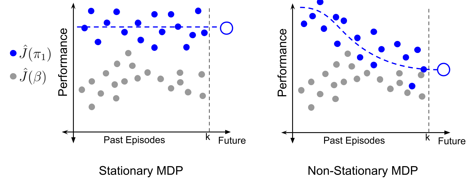
The above images illustrate the key idea. In a stationary environment, since the performance of \(\pi\) is constant across episodes, off-policy evaluation provides a noisy estimate about a constant value for \(\pi\)’s past performances. In comparison, in a non-stationary setting, off-policy evaluation provides a noisy estimate about a time-varying value for \(\pi\)’s past performances. Therefore, irrespective of the domain complexity, \(\pi\)’s future performance \(J_{k+1}(\theta)\) can now be forecasted using a univariate time series function \(\Psi\) that takes as input the counter-factual performance estimates for the past episodes,

\[\begin{align} \hat J_{k+1}(\theta) := \Psi (\hat J_1(\pi), \hat J_2(\pi), ...., \hat J_k(\pi)). \label{eqn:forecaster} \end{align}\]

Here is a simple example using least-squares regression. Let \(X := [1, 2, ..., k]^\top \in \mathbb{R}^{k \times 1}\) and \(Y := [\hat J_1(\pi), \hat J_2(\pi), \hat J_2(\pi), ..., \hat J_k(\pi)]^\top \in \mathbb{R}^{k \times 1}\), where \(k\) is the number for the last episode observed. Since performance trends need not be linear, let \(\phi(x) \in \mathbb{R}^{1 \times d}\) denote a \(d\)-dimensional basis function (e.g., Fourier basis) for encoding the time index, and \(\Phi\) be the corresponding basis matrix, such that non-linear performance trends can be captured. Then an estimate of \(\pi\)’s future performance can be obtained as

\[\begin{align} \hat J_{k+1}(\pi) = \phi(k+1)(\Phi^\top \Phi)^{-1}\Phi^\top Y. \end{align}\]

Note that this approach naturally generalizes for the stationary setting as well, where the time series trend essentially corresponds to a horizontal line.

Optimizing the future performance

Using the time-series perspective, we saw how future performance of a given policy \(\pi\) can be estimated. Now, to search for a policy that would maximize the future performance, we take a differentiable programming perspective and treat least-squares regression as a differentiable operator.

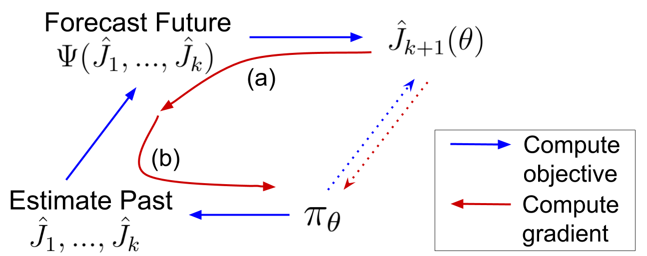
The above image illustrates the main idea. The dotted lines represent that we cannot use conventional methods to compute or estimate gradients of \(\hat J_{k+1}(\theta)\) as we have no samples from the future MDP. Instead, we estimate \(J_{k+1}(\theta)\) as a composition of two programs: one which connects the policy’s parameters to its past performances, and the other which forecasts future performance as a function of these past performances. An optimization procedure can be obtained by taking derivatives through this composition of programs to update policy parameters in a direction that maximizes future performance.

\[\begin{align} \frac{ d \hat J_{k+1}(\theta)}{d \theta} &= \frac{d \Psi(\hat J_1(\theta), ..., \hat J_k(\theta))}{d \theta} \\ % &= \sum_{i=1}^k \underbrace{ \frac{\partial \Psi(\hat J_1(\theta), ..., \hat J_k(\theta))}{\partial \hat J_i(\theta)}}_{\text{(a)}}\cdot \underbrace{ \frac{d \hat J_i(\theta)}{d \theta}}_{(b)}. \,\,\, \end{align}\]

This decomposition has an elegant and intuitive interpretation. The terms assigned to \((a)\) correspond to how the future prediction would change as a function of past outcomes, and the terms in \((b)\) indicate how the past outcomes would change due to changes in the parameters of the policy \(\pi_\theta\). Here, term (b) can be obtained using standard off-policy gradient estimators and term (a) can be obtained as the following,

\begin{align} \frac{\partial \hat J_{k+1}(\theta)}{\partial \hat J_i(\theta)} &= \frac{\partial \phi(k+1)(\Phi^\top \Phi)^{-1}\Phi^\top Y}{\partial Y_i}
% = [ \phi(k+1)(\Phi^\top \Phi)^{-1}\Phi^\top ]_i. \end{align}

Computationally, calculating \((\Phi^\top \Phi)^{-1}\) is also cheap as \((\Phi^\top \Phi)^{-1} \in \mathbb{R}^{d\times d}\), where \(d\) is the dimension of the basis and is extremely small compared to the number of data-points.

An intriguing behavior

In the equation for the total derivative above, notice that as the scalar term (a) is multiplied by the off-policy gradient term (b), the gradient \(d \hat J_{k+1}(\theta)/d \theta\) can be viewed as a weighted sum of off-policy policy gradients. To understand these weights better, in the left of the following figure we provide a visualization for the weights obtained from term (a) for different episodes \(i \in [1, 100]\).

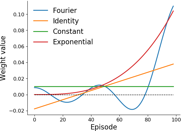
Perhaps intriguingly, when an identity basis or Fourier basis is used for \(\phi\), we notice an occurrence of negative weights, suggesting that the optimization procedure should move towards a policy that had lower performance in some of the past episodes!

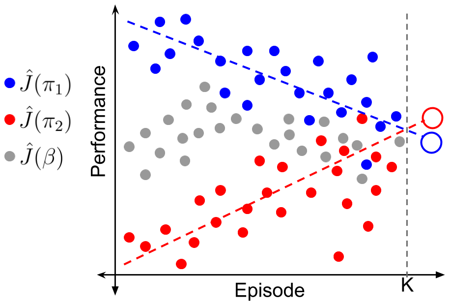
While this negative weighting seems unusual at first glance, it has an simple interpretation in hindsight. Consider the image on the right above. Despite having lower estimates of return everywhere, \(\pi_2\)’s rising trend suggests that it might have higher performance in the future, that is, \(J_{k+1}(\pi_2) > J_{k+1}(\pi_1)\). However, existing online learning methods like follow-the-leader maximize performance on all the past data uniformly (i.e., the green curve in the left image which gives equal weight to each episode). Similarly, the exponential weights (red curve in the left image) are representative of approaches that only optimize using data from recent episodes and discard previous data. It can be checked that either of these methods that use only non-negative weights cannot capture the trend to forecast \(J_{k+1}(\pi_2) > J_{k+1}(\pi_1)\).

In comparison, the weights obtained when using the identity basis (orange curve in the left image) would facilitate minimization of performances in the distant past and maximization of performance in the recent past. Intuitively, this means that it moves towards a policy whose performance is on a linear rise, as it expects that policy to have better performance in the future. Fourier basis further extends this idea while removing the restriction on the trend to be linear. Observe the alternating sign of weights in the figure above when using the Fourier basis. This suggests that the optimization procedure will take into account the sequential differences in performances over the past, thereby favoring the policy that has shown the most performance increments in the past. Further, these weights are obtained automatically as a by-product of regression!

Going Further

• One of the key drawbacks of using importance sampling is the variance resulting due to it. To mitigate variance, a popular method in stationary setting is to use weighted importance sampling (WIS). We show in our paper, that the idea of WIS can also be extended to non-stationary settings to significantly reduce variance. We encourage interested readers to check out more details and empirical results in the paper.

• There have been several recent works in RL that provide better off-policy estimates, and at the same time, there is an extensive literature on analyzing non-stationary time-series data. While we took the preliminary steps in this framework to bring these two communities closer, we believe there is a lot more that can be done here.

• In another blogpost, I discuss our NeurIPS 2020 work that takes an initial step towards further bridging ideas from the time-series literature to provide safe policy-improvement in non-stationary MDPs.